©
Optimal facility location (continuous)
  Finds the optimal location of a facility, the source, for minimum total cost of transportation to given destinations.
2024.Jul.03 12:38:06
n (2 ≤ |n| ≤ 20) No. of destinations, < 0 for a generated regular polygon¹ ('RP'). •
Context:  Case 1 -- pentagon Lisboa/Setúbal/Évora/Santarém/Leiria
Q
[kg] (If 0, Qi equal)
Capacities, Qi, or "weights" (demand at each destination, such as: item, kg, m³). •
C
[$ ⁄ kg-km] (If 0, C = 1)
Unit transportation cost (or made ≡ 1). (If circuity factor², use e.g. 1.3–1.6.) •
Coords. [km] (0 for RP) Points' coordinates, given as (xi, yi), i = 1..n (generated, for RP). •
itmax, tol, monit Iterations (max.), tolerance for (final) cost, monitoring (for iterative minimization). •
Show values Shows the coordinates of the graph.
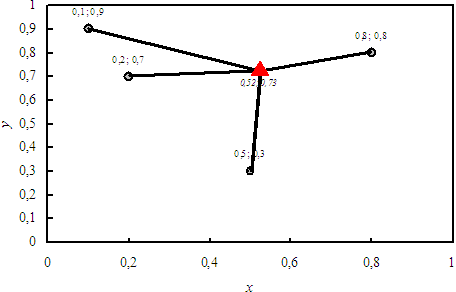
  Finds the optimal location, with coordinates X, Y, of a facility, P (red triangle in the Figure) —the source—, so as to minimize z, total cost of transportation to all the given destinations (4 points in the Figure), these requiring given quantities of goods, the capacities, Q, at given unit costs, C. (Direction of flow is immaterial.)
  The coordinates of P (X and Y) are assumed continuous. (An alternate, discrete strategy would be to give a set of candidate locations to optimize from.) Point P is found by a minimization method.
  A graph of the source coordinates and minimum cost —X, Y and z*— is made versus Q1 varying from 0 % to 100 % (of ∑iQi). Remark that the final result must obviously be z = 0, and, for an RP (see '¹', below), (X, Y) = (1, 0).
optiloc

¹ If n < 0, the destinations are the |n| vertices of a generated regular polygon (RP) inscribed in a unit circle, counterclockwise, with first point (+1, 0).

² (Suggested values.) The "circuity factor" is the quotient 'real distance' ⁄ 'straight line distance'.

Examples  n = −5 (1 1 1 1 1) → (3.078 1 1 1 1); [Francis & White, 1974]: (p 189) n = 4, Q = (1, 1, 1, 1), C ≡ 1, Coords = (0,0, 0,10, 5,0, 12,6) → P = (4, 2); (p 205, Pr. 4.29-a) n = 3, Q = (1, 3, 1), C ≡ 1, Coords = (0,0, 2,0, 0,2) → P = (2, 0), see the graph. [Love et al., 1988]: (p 17, Exa. 2.2) n = 4, Q = (1, 2, 2, 4), C ≡ 1, Coords = (1,1, 1,4, 2,2, 4,5) → P ≅ (2.6, 3.8), z = 195.76 (× 9⁄100 = 17.618)

NB: if using Internet Explorer, some symbols may not show (such as "approximately equal").
References:  (main bibliography...) Plate: NewOptiLocCont

• Search Fermat Weber location problem

• Weisstein, Eric W., "Minimum", from MathWorld —a Wolfram Web Resource.

• Hutt, Michael F., Programming, Nelder-Mead Simplex Fortran 90.

• Dennis, Jr., J. E., and Robert B. Schnabel, 1996, "Numerical methods for unconstrained optimization and nonlinear equations", SIAM, Philadelphia, PA (USA). Google browse. ISBN 0-89871-364-1 (pp 168–174.pdf).

• Burden, Richard L. and J. Douglas Faires, 1997, 6.th. (2004, 8.th) ed., "Numerical analysis", Brooks/Cole Publishing Company, Pacific Grove, CA (USA). Google browse. ISBN 0-534-95532-0 (pp 607 ff.).

• Biegler, L. T. (research group): nonlinear equations.pdf (=) ← courses, 06-720 AdvProcSysEng.ing (Carnegie Mellon Univ.).

• Ortega, J. M. and W. C. Rheinboldt, 1970, "Iterative solutions of nonlinear equations in several solutions", Academic Press, London (UK). Google browse. ISBN 0-12-528550-7 (pp 189–200: secant methods.pdf).

• Walton, Andrew G.: Solution of nonlinear algebraic equations.pdf (=), Imperial College London.

• Mathews, John H., 1987, "Numerical methods for computer science, engineering, and mathematics", Prentice-Hall, Inc., Englewood Cliffs, NJ (USA). Google browse. ISBN 0-13-626656-8. Broyden's method.

• 1867-11-03: Kutta, Martin Wilhelm (1944-12-25).