IST Vector Postprocessor

Pipeline

One pipeline

Solver output is rarely ready to plot: stresses arrive piecewise-constant on elements, displacements on nodes, tensors as nine loose scalars, and every field carries discretisation noise. IST Vector treats all of it as one pipeline, so the view on screen and the exported file do not diverge.

• Recovery is applied first. Switch on SPR and the colour bar, the iso-surfaces, the threshold mask and the deformation magnitudes all read the recovered field, so smoothed colour is not laid over unsmoothed data.
• One scene, four outputs. Screen, PDF, MP4 and saved state share the same scene object, so what the exporters write is what the viewport showed.
• Resolution-independent throughout. PDFs are shaded-triangle vector graphics rather than screenshots, MP4s capture the viewport’s physical pixel grid, and HiDPI displays are honoured end to end.

Screenshots

One model, several representations

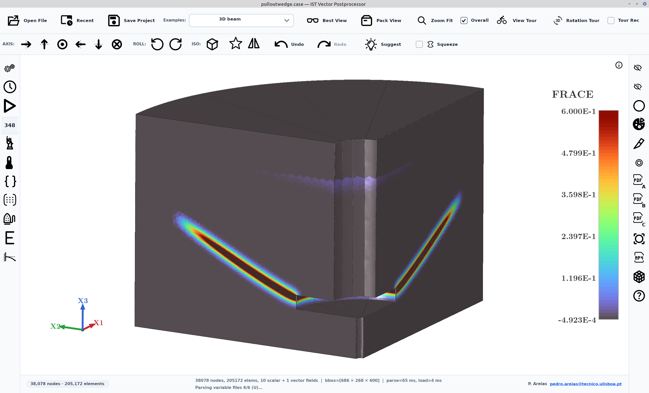
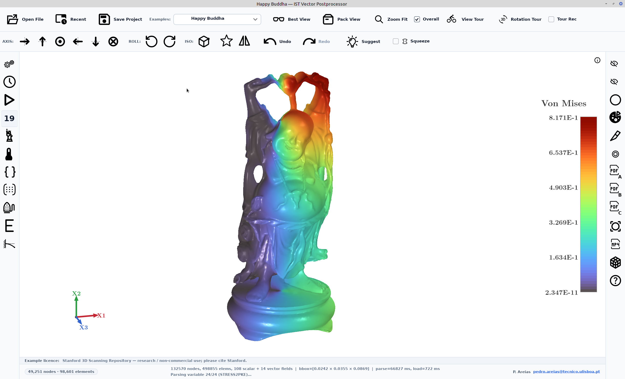
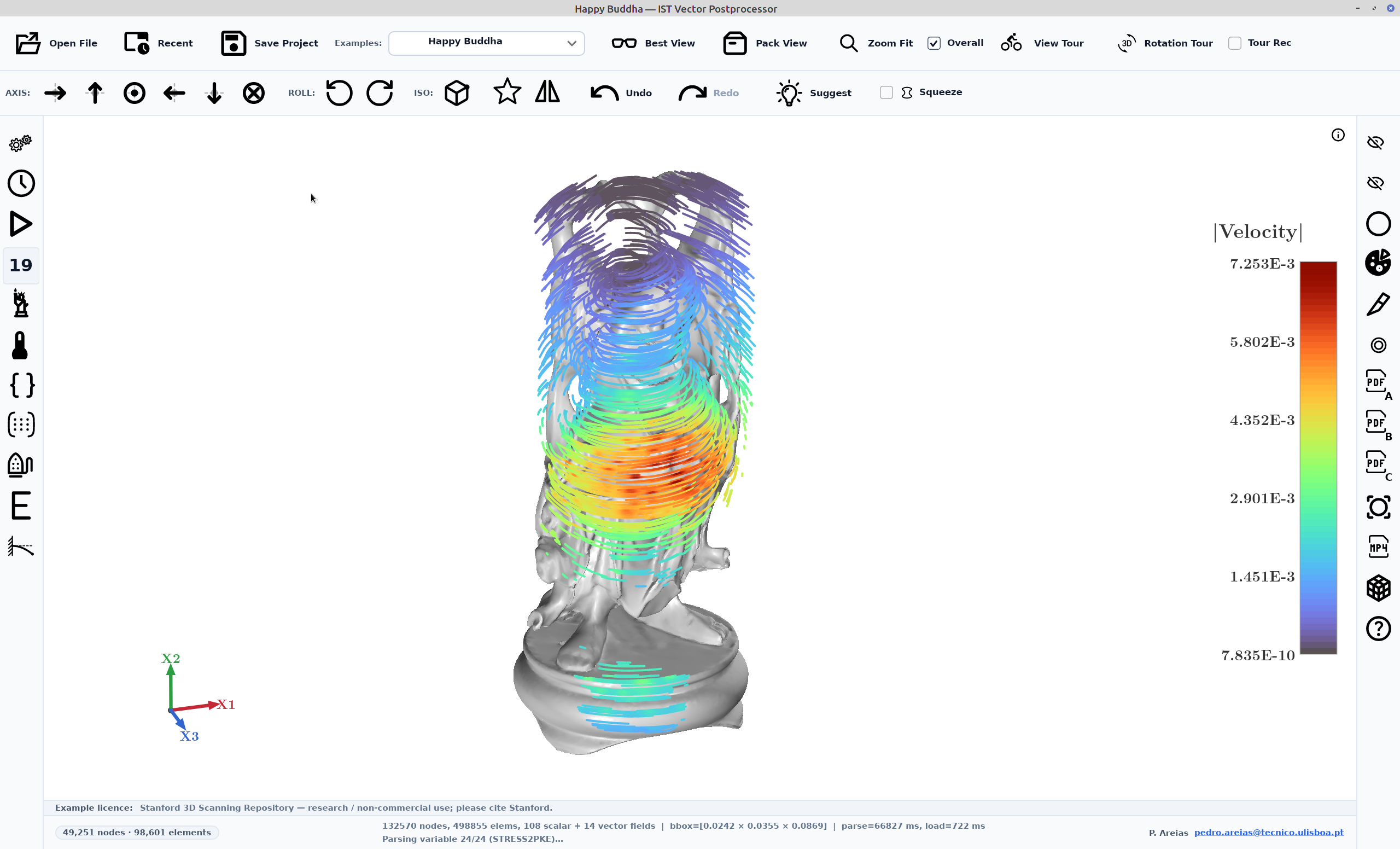
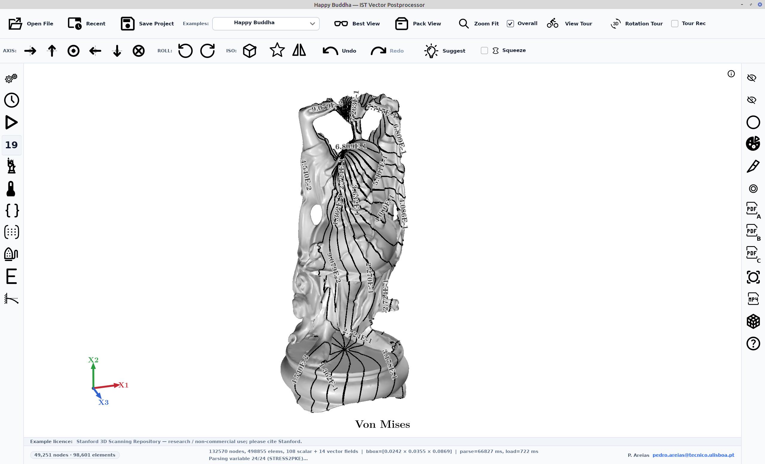
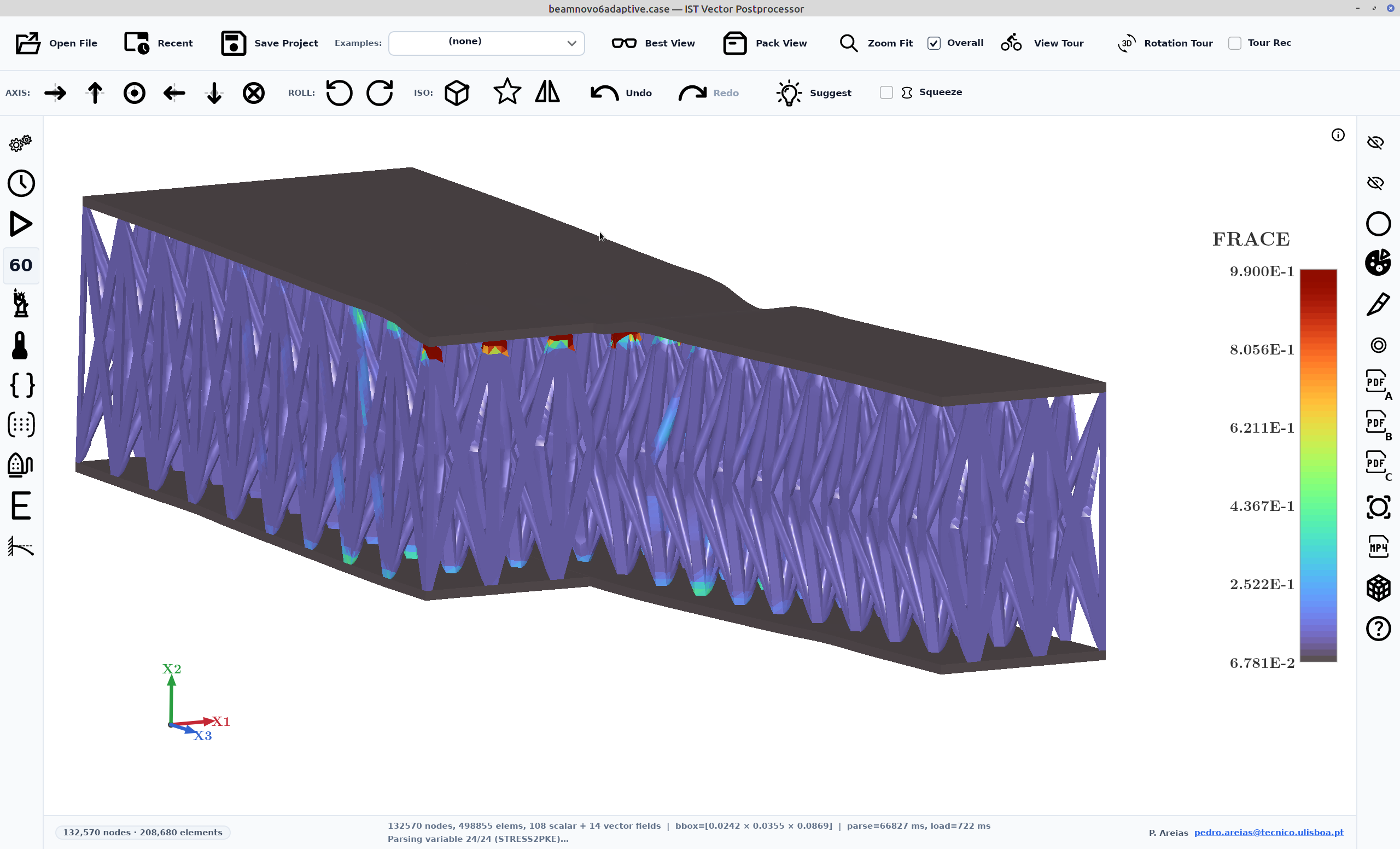
The bundled Stanford Happy Buddha in three representations (colour field, streamlines, print-mode iso-lines) and the fracture field from a lattice-beam damage run. Click any image for the full-size version; each scene exports as it stands to PDF and MP4. The Happy Buddha model is © Stanford University Computer Graphics Laboratory, from the Stanford 3D Scanning Repository, credited as its terms require.

Formats

Reads what your solver writes

Fields may be nodal or per-element; scalar, vector or tensor; steady or transient. Format detection reads the leading bytes of the file, so a mislabelled extension still reaches the right parser. Files open by drag-and-drop, by Ctrl+O, or from the recent-files flyout.

Element types

Every parsed cell collapses to one of these eight corner-only types; quadratic mid-edge and mid-face nodes are read past and discarded. VTK strips are unrolled, polygons with five or more vertices are fan-triangulated, VTK_VOXEL and VTK_PIXEL corner order is corrected, and structured grids unroll to hexa8 (or quad4 for slabs). General polygons and polyhedra (nsided, nfaced) are read but not rendered, and ghost cells are skipped. A node-only point cloud draws its nodes as round dots at a diameter you choose (the same in the live view, the PDF and the MP4), and the RBF recovery filter smooths fields over it.

Your own data

Write your data in a compatible format

If your solver, script or notebook writes none of the formats above, it does not have to learn one. ist_ensight_gold.py is a Python module shipped with IST Vector whose job is exactly that conversion: hand it your nodes, your element connectivity and your fields, and it writes a complete EnSight Gold data set (a .case file with its .geo geometry and one sidecar per field) that the postprocessor opens directly. EnSight and ParaView read the same output.

The whole interface is one function

from ist_ensight_gold import write_ensight_gold

write_ensight_gold(
    "out/beam.case",
    nodes=[(0, 0, 0), (1, 0, 0), (1, 1, 0), (0, 1, 0)],
    elements={"quad4": [(0, 1, 2, 3)]},
    node_data={"temperature": [20.0, 35.0, 50.0, 35.0]},
)

That writes out/beam.case, out/beam.geo and one file per field. Open the .case in IST Vector. Everything beyond this (several element blocks, several parts, transient steps, binary output) is another keyword on the same call.

What it accepts

Non-finite values (NaN, ±∞) are written as 0.0, since EnSight Gold cannot represent them; field and part names are sanitised, because the format cannot parse a name containing whitespace. Bad input raises EnSightError naming the offending field rather than producing a file that will not load. Run python ist_ensight_gold.py <directory> with no code of your own to write a small transient two-part demo data set and open that first.

Capabilities

From loaded field to finished figure

Ordered roughly as they are met in a session, from the recovery filter applied at load to the probes and camera tours used once a figure is ready.

Exports

What the scene can produce

Examples

Example exports

Dataset credits: Happy Buddha and Armadillo models © Stanford University Computer Graphics Laboratory, from the Stanford 3D Scanning Repository. Stanford permits research use and published images provided credit is given to the Stanford Computer Graphics Laboratory; commercial use of the models requires Stanford’s permission. 2-D pressure field: pyvista/vtk-data (Apache-2.0), originally from VTK’s test suite (BSD-3-Clause). Everything else is the author’s own finite-element results and procedurally generated surfaces.

Performance

Scale and performance

Strategy is selected from the mesh size, not configured. The tiers, and what changes at each:

Case bundles load fully into memory when the file total fits in 85% of available RAM; larger transients stream lazily: step 0 up front, while a field-major background preloader brings in the displayed fields across every step, so playback swaps in resident arrays instead of parsing from disk.

Representative costs

Mostly from the Reference Manual §7.2. ASCII .case decoding is newer than the manual: byte-level kernels, chunk-parallel across cores, put a 271 MB transient of 239 files (7 steps × 33 variables) at about 0.2 s of parsing rather than 2.2 s. During rotation and zoom the viewport renders to a half-resolution buffer and upscales, returning to full resolution on release. NaN and ±∞ are skipped in every reduction, so one bad sample does not collapse a colour range or hide the mesh.

Limitations

Limitations and requirements

Stated here rather than left to be discovered; most carry their workaround in the same sentence.

• Windows only. Windows 10 21H2 or Windows 11, x64, on a CPU meeting the x86-64-v2 baseline (SSE 4.2 and POPCNT); a startup preflight checks this and reports a failure. There is no macOS or Linux build. Displays from 1280×768 to 7680×4320 are supported.
• 15 GB of RAM or more recommended. Below that the application says so at startup and runs large transients in lazy-streaming mode rather than refusing them.
• A postprocessor, not a solver. It displays results; it does not compute them. Bring output from your own solver, or start from one of the bundled example datasets.
• Contours need nodal data. Per-element fields colour whole elements, and contours are never invented from them. Apply a recovery filter to move the field to nodes first, and everything downstream follows.
• Corner nodes only. Quadratic elements load, but mid-edge and mid-face nodes are read past, so display and export use the corner-only element. General polygons and polyhedra (nsided, nfaced) load but are not rendered.
• Meshes above 50 million nodes are declined at load, with the reason stated, rather than accepted and then thrashing.
• STL and OBJ carry geometry only. Useful as reference shapes; fields must come from an EnSight or VTK file.

Engineering

Engineering notes

• A headless core. The parsers, the recovery mathematics, the scene builder, the software rasteriser and the PDF writer live in a library that needs neither a window nor a GPU, so the whole pipeline can run, and be tested, without a display. The vector writer is written here rather than delegated to GL2PS or a similar OpenGL feedback-buffer library.
• Reproducible output. Depth sorting and shading are byte-stable, so PDF and frame output reproduce across runs and thread counts, and regression tests compare against pinned baselines.
• Tested against real solver output. The suite runs a corpus of EnSight, VTK, OBJ and STL files on every push, alongside fuzz fixtures: truncated, mislabelled and non-finite input.
• Playback allocates nothing per tick. Field interpolation alternates two scratch buffers, and coordinates are stored structure-of-arrays so hot loops stream one component at a time.
• Native AOT. A self-contained, fully trimmed executable, with source-generated JSON for all persistence, written atomically. OpenGL calls stay on the UI thread, and GPU caches rebuild from generation counters rather than explicit invalidation.
• Signed and timestamped. Release builds are Authenticode-signed with an Individual Validation (IV) code-signing certificate through signtool (SHA-256 file digest) and RFC 3161 countersigned, with DigiCert, Sectigo and GlobalSign timestamp fallback. The desktop executable, the first-party DLLs and the installer are each signed, so the signature still verifies after the certificate expires and SmartScreen passes the download without a warning.

Documentation

Manuals

How to cite

If figures made with IST Vector appear in a publication, cite the software itself and give the build date, so the version that produced them stays identifiable:

Datasets carry their own terms independently of this: scenes built on the Stanford models must keep the attribution the Stanford 3D Scanning Repository requires, which the PDF exporter prints with the figure.