To better describe the project let’s start with the Problem Definition:
Install a 3D LiDAR to detect objects in 3 Dimensions to improve 2D Navigation of an autonomous domestic mobile robot.
The project involves developing a navigation system for domestic robots (students used a TIAGo robot) using 3D sensors instead of traditional 2D ones. While 2D sensors may have limitations, such as not capturing the z coordinate, 3D sensors, like the Ouster OS1 LiDAR, overcome these limitations, enabling more precise and safe indoor navigation.
Those who might benefit from our project include robot manufacturers seeking to implement this solution/technology. Specifically, other robots encountering similar challenges as those to be further described. Additionally, elderly individuals or those with disabilities or illnesses stand to benefit from the robot’s focus on a domestic environment.


As demonstrated in the images above, a map with a 3D point cloud provides significantly more detail and information compared to a 2D map. To gain a better understanding of what a point cloud is, consider the following example: a robot captures the legs of a chair and a table using a 2D LiDAR.

Navigation using 2D LiDARs in domestic environments generally functions adequately but swiftly encounters the limitations of this technology. Consider, for example, the one-legged table in the image above; if the top is too large, the robot will collide with it. The same principle applies to various types of furniture, and 3D LiDARs overcome these barriers, ensuring easier autonomous navigation for the robot amidst static and dynamic obstacles, thus enhancing efficiency and precision.
Given that the project is part of the SocRob@Home team within the Institute For Systems and Robotics (ISR), it is crucial to emphasize what has already been accomplished and what we intend to undertake with our project.

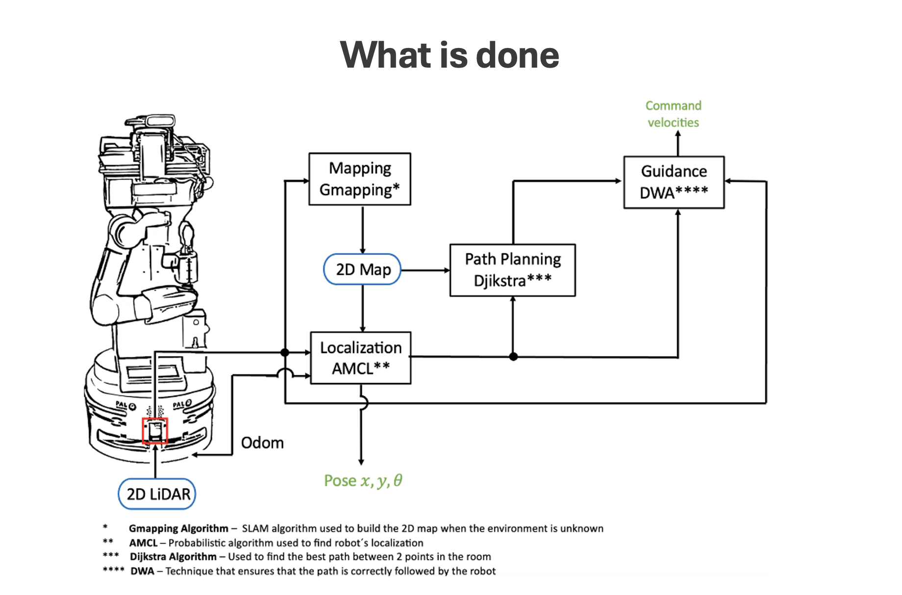
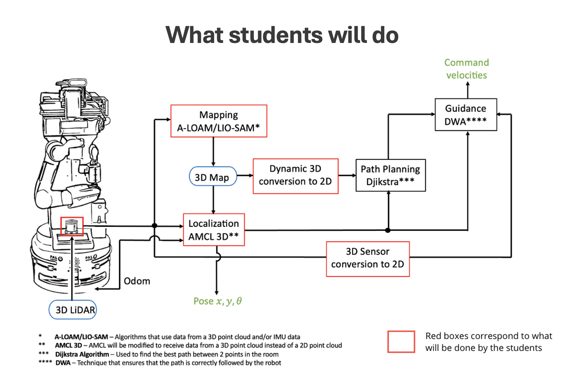
Figure 5 - What is already done by SocRob@Home and what students will develop
Figures 4 and 5 indicate that the subsequent navigation tasks will be developed:
-
3D Mapping
The current mapping method utilized is called Gmapping , a 2D SLAM algorithm that computes a 2D map, as demonstrated in Figure 1. The team is slated to evaluate two 3D SLAM algorithms (A-LOAM and LIO-SAM ), which will generate 3D maps as representations of the environment, akin to the one depicted in Figure 2.
-
3D Localization
The 3D localization will be achieved by researching alternative algorithms to AMCL. Existing algorithms capable of capturing a 3D point cloud from the Ouster OS1 LiDAR will be adapted. The objective is to test at least two options in simulation and determine which one is optimal for proceeding with real tests on the robot.
-
2D Path Planning/Guidance
This task involves converting the 3D point cloud acquired by the Ouster Sensor into obstacles on a 2D map. This conversion will be achieved by modifying an existing ROS node to discard points above the robot’s current height. Additionally, we’ll develop a new node to constantly update the robot’s footprint based on its arm position. This task ensures full compatibility of the 3D Ouster Sensor with existing path planning and guidance algorithms.
To ensure successful implementation, the robot must demonstrate confident movements to ensure safety for both individuals and objects. Additionally, it should be capable of accurately and efficiently sensing the 3D environment with a resolution of at least 5cm (ideally 2.5cm). Given that the current 2D navigation method yields a map resolution of 5cm, maintaining this feature is of particular interest. Furthermore, there should be a favorable balance between the benefits of utilizing a 3D sensor and its associated costs within the application.
Another solution requirement is the robot’s decision time to react to a dynamic obstacle and avoid a collision, that can is approximated by:
\[\tau = \frac{d}{v} - \frac{v}{a}\] where:
- 𝜏 - Robot’s decision time in seconds
- 𝑑 - Distance between TIAGo and an obstacle in meters (1.5m)
- 𝑣 - Robot’s velocity in meters per second (limited to 0.5m/s)
- 𝑎 - Robot’s max decelaration in meters per second squared (equal to -0.2m/s2)
Having explained this, one can now see how the decision time varies in function of distance and velocity in Figure 6.

The graph on the right is an enlargement of the one on the left in the zone of values of greater interest - shorter distances. When the decision time is equal to zero, it indicates that the robot will collide with an obstacle. Therefore, for a maximum velocity of 0.5m/s and an arbitrary distance of 1.5m, the decision time is 0.5 seconds. It will be tested whether the decision time is obtained for the corresponding velocity and distance values during the development of the project.
To test and validate the metrics, the students will assess every module both in simulation and in a real environment, utilizing a TIAGo robot as mentioned previously.

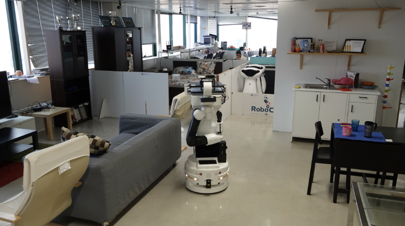
Figure 7 - Testbed simulation and real testbed
The tests will consist in navigation:
- In the testbed to a random waypoint without dynamic obstacles.
- In the testbed to a random waypoint with a dynamic obstacle (e.g., a person walking).
- In the testbed to a random waypoint with a small obstacle that 2D navigation does not avoid (e.g., sponge).
- From the kitchen to the living room, ensuring the robot avoids complex 2D navigation furniture (e.g., tables with center legs, chairs without back legs).
The students will repeat each experiment 5 or 10 times, record collisions and successes, and conduct a statistical analysis for both the current method and the one developed by the PIC1 team.
It is important to know that the methods currently in use involve the following frequency levels:
- Localization - 10Hz
- Path Planning - 2Hz
- Guidance - 10Hz
Furthermore, the students will compare the frequency levels obtained with the tested methods with those mentioned above.
One final test consists on evaluating the precision of the Localization with a Motion Capture System, based on 12 OptiTrack PRIME13 cameras that have a sub-millimeter precision. The error obtained will be compared with the error of the current method used (AMCL - with 0.09 meter accuracy).
